A small programming exercise in APL #2: Combinations

In this post I'm going to continue my APL exploration by working in a possible solution for the problem of generating all the combinations of 'n' elements of an array.

Generating the 'n' combinations of an array means generating a sequence of all possible 'n' unique elements from the original array . For example, given the array 12, 34, 35, 65 all possible '2' combinations of this array are:

• 12, 34
• 12, 35
• 12, 65
• 34, 35
• 34, 65
• 35, 65

Notice that order is not important. That is "12, 34" is considered to be the same as "34, 12". Generating all 'n' permutations of the elements of an array may be an interesting problem for a future post.

One of my goals was to be as idiomatic as possible (with my limited APL knowledge!). Because of this, I will try avoid using explicit loops or conditionals and instead use array operators.

Strategy

The general strategy for solving this problem was to calculate all possible boolean arrays having 'n' bits and use Compress to extract the elements.

For example, in the array 12, 34, 35, 65 all possible boolean vectors having two bits on are:

• 1 1 0 0
• 1 0 1 0
• 1 0 0 1
• 0 1 1 0
• 0 1 0 1
• 0 0 1 1

Using these vectors in APL we get the elements we need:

      a
12 34 35 65
      1 1 0 0 / a
12 34
      1 0 1 0 / a
12 35
      1 0 0 1 / a
12 65
      0 1 1 0 / a
34 35
      0 1 0 1 / a
34 65
      0 0 1 1 / a
35 65

This strategy is not efficient in space or time but it allowed me to explore a solution without using imperative constructs or recursion.

Generating the boolean arrays

To generate the boolean arrays we start by generating all integer values required to encode n-bit values:

      a ← 12 34 35 65
      ⍳ ( ¯1 + 2 * ⍴ a)
1 2 3 4 5 6 7 8 9 10 11 12 13 14 15

When converting these numbers to binary we get all possible boolean vectors for 4-bit values. This is same as the same as the length of our sample array. We can see these arrays if we use Encode and Each:

     { ((⍴ a) ⍴ 2) ⊤ ⍵ } ¨ ⍳ ( ¯1 + 2 * ⍴ a)
 0 0 0 1  0 0 1 0  0 0 1 1  0 1 0 0  0 1 0 1  0 1 1 0  0 1 1 1  1 0 0 0\
  1 0 0 1  1 0 1 0  1 0 1 1  1 1 0 0  1 1 0 1  1 1 1 0  1 1 1 1

I can reshape this array to get a better representation:

      15 1 ⍴ { ((⍴ a) ⍴ 2) ⊤ ⍵ } ¨ ⍳ ( ¯1 + 2 * ⍴ a)
 0 0 0 1
 0 0 1 0
 0 0 1 1
 0 1 0 0
 0 1 0 1
 0 1 1 0
 0 1 1 1
 1 0 0 0
 1 0 0 1
 1 0 1 0
 1 0 1 1
 1 1 0 0
 1 1 0 1
 1 1 1 0
 1 1 1 1

Now we are only interested in boolean arrays with 'n' number of '1' bits. For n = 2 we can get only those elements using the Compress operator:

      seq ← ⍳ ( ¯1 + 2 * ⍴ a)
      n ← 2
      ({ n =  +/ ((⍴ a) ⍴ 2) ⊤ ⍵} ¨ seq) / seq
3 5 6 9 10 12

Again we can visualize these values using reshape and encode:

      6 1 ⍴ { ((⍴ a) ⍴ 2) ⊤ ⍵ } ¨ ({ n =  +/ ((⍴ a) ⍴ 2) ⊤ ⍵} ¨ seq) / seq
 0 0 1 1
 0 1 0 1
 0 1 1 0
 1 0 0 1
 1 0 1 0
 1 1 0 0
 

Selecting desired elements

Now that we have our boolean arrays we can pick all the values using Compress:

     {(((⍴ a) ⍴ 2) ⊤ ⍵)/a} ¨ ({ n =  +/ ((⍴ a) ⍴ 2) ⊤ ⍵} ¨ seq) / seq
 35 65  34 65  34 35  12 65  12 35  12 34

And again we can reshape this array to see it better:

      6 1 ⍴ {(((⍴ a) ⍴ 2) ⊤ ⍵)/a} ¨ ({ n =  +/ ((⍴ a) ⍴ 2) ⊤ ⍵} ¨ seq) / seq
 35 65
 34 65
 34 35
 12 65
 12 35
 12 34

Finally we can pack these expressions in a function:

∇r←a ncombinations1 n;seq
  seq ← ⍳ ( ¯1 + 2 * ⍴ a)
  r ← {(((⍴ a) ⍴ 2) ⊤ ⍵)/a} ¨ (({ n =  +/ ((⍴ a) ⍴ 2) ⊤ ⍵} ¨ seq) / seq\
)
∇

We can use it like this:

      1 2 3 4 5 ncombinations1 3
 3 4 5  2 4 5  2 3 5  2 3 4  1 4 5  1 3 5  1 3 4  1 2 5  1 2 4  1 2 3

APL has a build-in Binomal operator which allows us to calculate the number of combinations. For example:

      a ← 1 2 3 4 5
      (3 ! ⍴ a) = ⍴ a ncombinations3 3
1

Final words

It was very interesting (and difficult) to try to write a solution of this problem using only array operations. Reading the definion of the ncombinations1 I noticed that there are many expressions nested in parenthesis (maybe related to my limited APL knowledge). I know that APL developers value terseness, so I tried to reduce the size of the expressions. Here is a new version:

∇r←a ncombinations3 n;seq
  s ← ⍳ ( ¯1 + 2 * ⍴ a)
  b ← 2⍴⍨⍴a
  r ← {a/⍨b⊤⍵}¨s/⍨{n=+/b⊤⍵}¨s
∇

I was able to remove a couple of parenthesis by taking advantage of the Commute operator.

GNU APL was used to create the examples in this post.

A small programming exercise in APL #1

This post shows a possible solution written in APL for the following programming problem:

Given an array, determine if a value 'number' is found in every consecutive segment of 'size' elements.

For example, given this array:

1,2,1,3,4,1

This predicate is true for number = 1 and size = 2. Because '1' is found in (1,2), (1,3) and (4,1).

A possible APL solution

This is a possible solution to this problem (using my limited APL knowledge).

∇ z←array arraysegments args
  number ← args[1]
  size ← args[2]
  z ← ∧/ ({number∊⍵} ⍤1) (((⍴ array) ÷ size) , size) ⍴ array
∇

This function is called arraysegments and is a dyadic function. It receives the array to validate as the left argument and on the right argument a two-value array with the value ('number') to find inside the array segment and the length of the segments.

An example of using this function

      1 2 1 3 4 1 arraysegments 1 2
1
      1 2 1 3 4 1 arraysegments 2 2
0
      1 2 1 3 4 1 arraysegments 1 3
1
      300 200 300 300 400 500 arraysegments 300 3
1
      300 200 300 300 400 500 arraysegments 400 3
0

To see how this function works I'm going to start by defining some sample data:

      array ← 1 2 1 3 4 1 
      number ← 1
      size ← 3

1. First, start by reshaping the input array into a matrix with each row being

      (((⍴ array) ÷ size) , size)
2 3      
      (((⍴ array) ÷ size) , size) ⍴ array
1 2 1
3 4 1

2. Now that we have the 'groups' as the rows of the new matrix, we apply the membership operation to each element of the matrix. To do this, we use the rank operator in conjunction with an inline function to test the membership:

      ({number∊⍵} ⍤1) (((⍴ array) ÷ size) , size) ⍴ array
1 1

As a final step we apply the reduce operator '/' with the And operator to see if the input number exists in every group:

      ∧/ ({number∊⍵} ⍤1) (((⍴ array) ÷ size) , size) ⍴ array
1

There are some problem with this solution. For example if the array cannot be splitted in groups of the specified size you get a runtime error.

Reading APL #1: Roman numerals to decimal

As part of a new recurring series I’m going to take a small APL function or program and try to break it down in to its parts. I hope this is going to help me get a better understanding of the language.

Reading APL

This article: The APL Programming Language Source Code has a nice introduction to the language and its history. One sentence in this article is key to understand how to read APL code:

Order of evaluation: Expressions in APL are evaluated right-to-left, and there is no hierarchy of function precedence

Two additional concepts are useful to understand when trying to read code:

1. A monadic function : an operation applied to the right expression
2. A dyadic function : a function applied to two arguments ( left and right )

One example of these elements is the following:

      2 2 ⍴⍳⍴ 8 8 8 8
1 2
3 4

Here is an example of evaluating this expression from right to left.

      myarray←8 8 8 8
      myarray
8 8 8 8
      length_of_my_array← ⍴ myarray
      length_of_my_array
4
      new_array← ⍳ length_of_my_array
      new_array
1 2 3 4
      2 2 ⍴ new_array
1 2
3 4

Note that here we use ⍴ both as a monadic function (Shape) and as a dyadic function (Reshape).

The example

For this post I’m going to use a small function I found in the APL Utils repository by Blake McBride . This function takes a string representing a roman number and converts it back to an integer:

∇z←Romanu a
 z←+/(¯1+2×z≥1↓z,0)×z←(1 5 10 50 100 500 1000)['IVXLCDM'⍳a]
∇

An example of executing this function:

      Romanu 'XVII'
17
      Romanu 'IX'
9

Reading the code

Let’s start by reading the function definition:

∇z←Romanu a
   ...
∇

This code represents the definition of the Romanu function with an a argument.

Now, the interesting part is reading the body of the function which performs the actual calculations.

z←+/(¯1+2×z≥1↓z,0)×z←(1 5 10 50 100 500 1000)['IVXLCDM'⍳a]

As described in the previous section we need to read this code from right to left. To do this we need to ‘parse’ it and extract the largest complete expression from the right:

(1 5 10 50 100 500 1000)['IVXLCDM'⍳a]

This expression is a particular example of an bracked indexing expression(https://aplwiki.com/wiki/Bracket_indexing). A simpler example of this is:

      (10 20 30)[1]
10
      (10 20 30)[2]
20
      (10 20 30)[3]
30
      (10 20 30)[3 1 1 2]
30 10 10 20
      a←10 20 30
      a[3 1 1 2]
30 10 10 20

As shown above this expression is used to select elements of an array into a new array.

In the Romanu function this expression is used to assign a value to eacho of the roman numeral 'digits':

'IVXLCDM'⍳a

Here the dyadic form of ⍳ or ‘Index of’(https://aplwiki.com/wiki/Index_Of) . This expression returns the indices of the left side array of the elements on the right. Here are some examples of this expression in action:

      (10 20 30) ⍳ (20 20 10 20 30 10)
2 2 1 2 3 1

When using this expression with the roman digits string we get the equivalent positions:

      'IVXLCDM' ⍳ 'XVII'
3 2 1 1

As shown above we get the positions in the roman digits string. Returning to our original expression we use the selection expression to get the value of each roman digit in decimal form:

      (1 5 10 50 100 500 1000)['IVXLCDM' ⍳ 'XVII']
10 5 1 1

As you can see here we almost have the result for the conversion of XVII. We just have to sum these numbers up to get 17.

Going back to the example and continuing reading for right to left we find and assignment to the z variable.

z←(1 5 10 50 100 500 1000)['IVXLCDM'⍳a]

The rest of the expression is going to take care of subtracting the value required for converting numbers like: ‘IX’.

Reading the expression from right to left we find:

(¯1+2×z≥1↓z,0)×z←(1 5 10 50 100 500 1000)['IVXLCDM'⍳a]

This expression is a multiplication (×). For arrays it applies to operation element wise :

      2 3 × 4 5
8 15

The interesting part here is the expression being used for the left operand of the multiplication:

(¯1+2×z≥1↓z,0)

Again we are going to analyze this expression from right to left.

z,0

This expression returns the an array with a zero at the end:

     (10 20 30),0
10 20 30 0
      z←(1 5 10 50 100 500 1000)['IVXLCDM' ⍳ 'IX']
      z,0
1 10 0

Then the following operation drops the first element of the array:

      1↓z,0
10 0

The drop expression returns an array without the first ‘n’ elements:

      3 ↓ 20 30 40 30 20 10
30 20 10

The following section is very interesting . We use the greater equal expression ≥ to determine which elements of the array are greater or equal than the second array:

       10 20 30 ≥ 5 21 30
1 0 1

Applying this to our example for ‘IX’:

      z←(1 5 10 50 100 500 1000)['IVXLCDM' ⍳ 'IX']
      z≥1↓z,0
0 1

This is interesting: we get an array that indicates which entries are lower than its successor. In the case of IX we are getting 0 1 saying that the first digit needs to be subtracted from the second. The final part performs this operation.

      z←(1 5 10 50 100 500 1000)['IVXLCDM' ⍳ 'IX']
      z≥1↓z,0
0 1
      ¯1+2×z≥1↓z,0
¯1 1
      (¯1+2×z≥1↓z,0)×z
¯1 10

Now we can finally sum all the numbers on the resulting array and get the decimal number. This is performed with the reduce operation / (https://aplwiki.com/wiki/Reduce) with the + operator.

      +/ 10 20 30
60
      10 + 20 + 30
60

Applying this operation to our partial expression returns the expected value:

      (¯1+2×z≥1↓z,0)×z
¯1 10

      +/(¯1+2×z≥1↓z,0)×z
9

We can see this process in action by executing all the parts with an interesting number like MMCXXIX (2129).

      z←(1 5 10 50 100 500 1000)['IVXLCDM'⍳a]
      z
1000 1000 100 10 10 1 10
      z,0
1000 1000 100 10 10 1 10 0
      1↓z,0
1000 100 10 10 1 10 0
      z≥1↓z,0
1 1 1 1 1 0 1
      ¯1+2×z≥1↓z,0
1 1 1 1 1 ¯1 1
      +/(¯1+2×z≥1↓z,0)×z
2129

A small Tetris-like clone using J and ncurses. Part 1

For me, the J programming language it's a very intriguing. It is full of ideas and concepts that I'm not familiar with. Getting to know a programming language it's not only about learning the syntax. It is learning the techniques that people use to take advantage of it what gives you more insight . This is particularly true for J.

For me the best way to learn more about a programming language is to try to solve a small problem with it. In this post I'm going to describe an attempt to write a small and incomplete Tetris-like clone using J and the ncurses library. Here's a preview of how it looks:

Tetriminos

According to the Wikipedia page for Tetris, the pieces are named Tetriminos https://en.wikipedia.org/wiki/Tetris#Gameplay. Each piece is composed of blocks. In J we can represent this pieces as matrices.

To create this matrices we use the Shape verb ($) For example:

• The "L" tetrimino:

   ] l_tetrimino =. 2 3 $ 1 1 1 1 0 0 
1 1 1
1 0 0

• The "O" tetrimino:

   ] b_tetrimino =. 2 2 $ 4 4 4 4 
4 4
4 4

• The "S" tetrimino:

   ] s_tetrimino =. 2 3 $ 0 5 5 5 5 0 
0 5 5
5 5 0

Tetrimino rotation

In Tetris pressing the 'up' arrow is going to rotate the current piece. We can use matrix Transpose (|:) and Reverse (|.) verbs and compose them together using the Atop conjunction (@). Here's the definition:

rotate =: |.@|:

Here we can see how this verb works:

   l_tetrimino
1 1 1
1 0 0
   rotate l_tetrimino
1 0
1 0
1 1
   rotate rotate l_tetrimino
0 0 1
1 1 1
   rotate rotate rotate l_tetrimino
1 1
0 1
0 1
   rotate rotate rotate rotate l_tetrimino
1 1 1
1 0 0

We can apply this transformation to the other tetriminos for example:

   ] s_tetrimino =. 2 3 $ 0 5 5 5 5 0 
0 5 5
5 5 0
   rotate s_tetrimino
5 0
5 5
0 5
   rotate rotate s_tetrimino
0 5 5
5 5 0

We use different numbers for each tetrimino so we can use different colors to paint them.

Tetrimino placement

A natural way to model the game is to use a matrix representing the playing field. We use a 10 columns by 20 rows matrix for this effect. We use the Shape verb ($) to do this:

   ] game =:  20 10 $ 0
0 0 0 0 0 0 0 0 0 0
0 0 0 0 0 0 0 0 0 0
0 0 0 0 0 0 0 0 0 0
0 0 0 0 0 0 0 0 0 0
0 0 0 0 0 0 0 0 0 0
0 0 0 0 0 0 0 0 0 0
0 0 0 0 0 0 0 0 0 0
0 0 0 0 0 0 0 0 0 0
0 0 0 0 0 0 0 0 0 0
0 0 0 0 0 0 0 0 0 0
0 0 0 0 0 0 0 0 0 0
0 0 0 0 0 0 0 0 0 0
0 0 0 0 0 0 0 0 0 0
0 0 0 0 0 0 0 0 0 0
0 0 0 0 0 0 0 0 0 0
0 0 0 0 0 0 0 0 0 0
0 0 0 0 0 0 0 0 0 0
0 0 0 0 0 0 0 0 0 0
0 0 0 0 0 0 0 0 0 0
0 0 0 0 0 0 0 0 0 0

A fundamental piece of functionality that we need is a way to put a tetrimino inside this matrix. This proved to be tricky (maybe because of lack of J knowledge). We're going to incrementally create this verb.

Reading the J documentation, it seems that we can use the Amend (m } _ _ _) verb to change just a set of cells of the game matrix. Here's an example on how to use this verb

   ] sample =. 5 5 $ 0
0 0 0 0 0
0 0 0 0 0
0 0 0 0 0
0 0 0 0 0
0 0 0 0 0

   1 2 3 4 (1 1;2 1;1 2;2 2) } sample
0 0 0 0 0
0 1 3 0 0
0 2 4 0 0
0 0 0 0 0
0 0 0 0 0

What we are saying here is that we can to change the following cells in sample:

• row 1 column 1 with value 1
• row 2 column 1 with value 2
• row 1 column 2 with value 3
• row 2 column 2 with value 4

Now to take advantage of this verb we need to calculate the target coordinates to change the value of a tetrimino. First we start by generating coordinates for each of the cells of the tetrimino.

We're going to use the following predifined values:

   ] l_tetrimino =. 2 3 $ 1 1 1 1 0 0 
1 1 1
1 0 0
   sample
0 0 0 0 0
0 0 0 0 0
0 0 0 0 0
0 0 0 0 0
0 0 0 0 0

We start by determining how many rows and columns. We use the Shape of verb ($) to do this:

   $ l_tetrimino
2 3

Now we want to generate (0, 0);(0, 1);...(1, 2);(2, 2). With the result of Shape of we generate a sequence of numbers for each of the axis. To do this we use the Integers (i.) verbwith the number of rows and the number of columns. For example:

   NB. Get the number of rows:
   (0&{@$) l_tetrimino
2
   NB. Get the number of columns:
   (1&{@$) l_tetrimino
3
   NB. Get an integer sequence from zero to number of rows or columns
   i.(1&{@$) l_tetrimino
0 1 2
   i.(0&{@$) l_tetrimino
0 1

Now this is very cool, we can use the Table verb (/)to pair this two arrays. From the documentation:

In general, each cell of x is applied to the entire of y . Thus x u/ y is equivalent to x u"(lu,_) y where lu is the left rank of u .

This is very important!. To taken advantage of this we need to use the Append verb (,) but changing the rack to operate on each of the elements from the right argument. See this example:

   0 (,"0) 0 1 2
0 0
0 1
0 2

Now we can take advantage of this and write:

   (  (i.@(0&{@$)) (<@,"0)/ (i.@(1&{@$))) l_tetrimino 
+---+---+---+
|0 0|0 1|0 2|
+---+---+---+
|1 0|1 1|1 2|
+---+---+---+

Now this is almost what we need. We can use the Ravel veb (,) to flatten this box:

, (  (i.@(0&{@$)) (<@,"0)/ (i.@(1&{@$))) l_tetrimino
+---+---+---+---+---+---+
|0 0|0 1|0 2|1 0|1 1|1 2|
+---+---+---+---+---+---+

With this positions we can use the Amend verb to change our game matrix:

   (,l_tetrimino) positions } sample
1 1 1 0 0
1 0 0 0 0
0 0 0 0 0
0 0 0 0 0
0 0 0 0 0

We need something else since this technique only allows us to put the tetrimino at the top of the matrix. In order to do this we need to sum the target position to the coordinates that we generated. We can use the powerful Under verb (&.) which allows us to apply an operation to each of the cells of a box.

   (3 2)&+ &.> positions
+---+---+---+---+---+---+
|3 2|3 3|3 4|4 2|4 3|4 4|
+---+---+---+---+---+---+

We construct this operation by:

1. using Bond conjuction (&) to tie together the position (3 2) with the plus operation (+) . That is (3 2)&+ .
2. we apply this operation to each of the elements of the box and then assemble the box again. That is &.>

Now we can put the tetrimino in row 3, column 2.

   target_position =. 3 2
   target_position =. 2 1
   (,l_tetrimino) (target_position&+&.>positions) } sample
0 0 0 0 0
0 0 0 0 0
0 1 0 0 0
0 1 1 1 0
0 0 0 0 0

We cannot just pust the tetrimino in the target position. It may also "blend" with existing values. For example say the following game field and the following tetrminio:

   ] game
0 0 0 0 0
0 0 0 0 0
0 0 0 1 0
0 0 0 1 0
0 0 0 1 1

positions =., (  (i.@(0&{@$)) (<@,"0)/ (i.@(1&{@$))) tetrimino

   (,tetrimino) ((1 2)&+&.> positions) } game
0 0 0 0 0
0 0 1 1 0
0 0 1 0 0
0 0 1 0 0
0 0 0 1 1

Because of this we need to mix the tetrimino with the current values of the target region. We do this by extracting the values of the target position:

   ($tetrimino) $ ((1 2)&+&.> positions) { game
0 0
0 1
0 1

We can combine this array with the tetrimino and we get the desired target value:

   ] target_tetrimino =. +&tetrimino ($tetrimino) $ ((1 2)&+&.> positions) { game
1 1
1 1
1 1

   (,target_tetrimino) ((1 2)&+&.> positions) } game
0 0 0 0 0
0 0 1 1 0
0 0 1 1 0
0 0 1 1 0
0 0 0 1 1

The final verb definition looks like this:

put_in_matrix =: 3 : 0
 NB. unpack argumets
 tetrimino =. > 0 { y
 i =. > 1 { y
 j =. > 2 { y
 game =. > 3 { y

 NB. calculate target positions 
 positions =. , ((i.@(0&{)@$)(<@,"0)/(i.@(1&{)@$)) tetrimino

 NB. combine tetrimino with target section
 tetrimino =. +&tetrimino ($tetrimino) $ ((+&(i,j))&.> positions) { game
  
 NB. change matrix
 (,tetrimino) ((+&(i,j))&.> positions)} game
)

Checking if space is available

The other piece of functionality that we need is a way to verify if we can put the tetrimino in a target position. We need to verify two conditions: 1. We can put the tetrimino inside the game field. 2. There's space available in the target position.

To check the boundaries we use common comparison operators:

 NB. Verify field boundaries
 is_inside =. (xpos >: 0) *. (ypos >: 0) *. ( (xpos+tetrimino_width - 1) < game_width) *. ((ypos+tetrimino_height - 1) < game_height)

The second criteria it's more intersesting. To illustrate how we did the detection we're going to start with a predifined game field:

   game
0 0 0 0 0
0 0 0 0 0
0 0 0 0 0
0 0 0 1 0
0 0 0 0 0
   ] tetrimino =. 2 3 $ 2 0 0 2 2 2
2 0 0
2 2 2

The first step is to reset the values of the tetrimino to be either zero or one:

   ] tetrimino =. 0&< tetrimino
1 0 0
1 1 1

Now we extract the elements of the target position (in this example column 1, row 3)

   ypos =. 3
   xpos =. 1
   positions =. , ((i.@(0&{)@$)(<@,"0)/(i.@(1&{)@$)) tetrimino
   ($tetrimino) $ ((+&(ypos,xpos))&.> positions){ game
   
0 0 1
0 0 0

   xpos =. 1
   ypos =. 2
   positions =. , ((i.@(0&{)@$)(<@,"0)/(i.@(1&{)@$)) tetrimino
   ($tetrimino) $ ((+&(ypos,xpos))&.> positions){ game
0 0 0
0 0 1

Now we can multiply the tetrimino by the target value:

   target_segment =. ($tetrimino) $ ((+&(ypos,xpos))&.> positions){ game
   ] hits =. +/ , *&tetrimino target_segment
1

Now the variable hits contains the number of elements with a target cell value. The final predicate looks like this:

can_put_in_matrix =: 3 : 0
 NB. Unpack the arguments
 tetrimino =. 0&< > 0 { y
 tetrimino_width =. 1 { $ tetrimino
 tetrimino_height =. 0 { $ tetrimino
 ypos =. > 1 { y
 xpos =. > 2 { y
 game =. > 3 { y
 game_width  =. 1 { $ game
 game_height =. 0 { $ game

 NB. Verify field boundaries
 is_inside =. (xpos >: 0) *. (ypos >: 0) *. ( (xpos+tetrimino_width - 1) < game_width) *. ((ypos+tetrimino_height - 1) < game_height)

 NB. Check if we hit an occupied cell
 hits =. 0
 if. is_inside do.
   positions =. , ((i.@(0&{)@$)(<@,"0)/(i.@(1&{)@$)) tetrimino
   hits =. +/ , *&tetrimino ($tetrimino) $ ((+&(ypos,xpos))&.> positions){ game
 end.

 is_inside *. (hits = 0)
)

End words

As it was said in the beginning, J it's very interesting. For me there are many things to learn (you can tell that by looking at all those parenthesis in some expressions). Also there are many strategies in array languages that one needs to understand in other to write idiomatic code.

The ncurses interface will be discussed in part 2. For future posts it will be interesting to talk about concepts like the obverse (http://www.jsoftware.com/help/jforc/u_1_uv_uv_and_u_v.htm#_Toc191734413) and state machines (http://www.jsoftware.com/help/jforc/loopless_code_vii_sequential.htm#_Toc191734470) .

Code for this post can be found here: https://github.com/ldfallas/jcurtris

A quick look at APL

In this post I'm going to show an implementation of polynomial multiplication written in APL and the steps to create it.

APL

APL is an array oriented programming language which means it's good for manipulating vectors, matrices and other kinds of arrays.

APL has many interesting characteristics among them is its syntax which uses non ASCII characters .

Here's a very nice video showing how to implement the Conway's Game Of Life in APL:



A very nice APL resource is the APL Wiki it has lots of information. Another very nice resource is The FinnAPL Idiom Library which contains lots little examples of code. Another nice resource is Vector the journal of the British APL Association which has information on the community around APL related languages.

The examples presented in this post were written using NARS2000 a nice open source implementation of APL.

Polynomial multiplication

As with a previous post on J I'm going to show the implementation of polynomial multiplication .

The following example shows the process of multiplying two polynomials:

(4x3 - 23x2 + x + 1) * (2x2 - x - 3)

= ((4x3 - 23x2 + x + 1) * 2x2) +
((4x3 - 23x2 + x + 1) * -x) +
((4x3 - 23x2 + x + 1) * -3)

= (8x5 - 46x4 + 2x3 + 2x2) +
(-4x4 + 23x3 - x2 - x) +
(-12x3 + 69x2 - 3x - 3)

= (8x5 - 50x4 + 13x3 + 70x2 - 4x - 3)

This example will be used to illustrate the parts of the code in the following sections.

The program

The final program to calculate polynomial multiplication looks like this:



Where a and b are the polynomials.

As with the previous post on J I'm sure there's a shorter way to write this program
(the number of parenthesis seems to indicate this!).

One key aspect to understand APL code is to remember that it evaluates expressions from right to left. See the Order of execution section of the APL Wiki for more information.

A description of each part of this program is presented in the following sections.

Polynomial representation

To represent polynomials we're going to use vectors the following way:

For:

(4x3 + 23x2 + x + 1)

the array will be:

1 1 23 4

In APL arrays are written as sequences of numbers separated by spaces (as above). You can manipulate this values easily, for example here we create two variables with two polynomials and add them:



In order to multiply each element of the array by a value we can simply write:

Outer product

The outer product operator lets you apply an operation to all the combinations of the elements of the operands. For example if we want to multiply each value of the two arrays representing the polynomials we want to multiply we can write:

Creating a matrix of intermediate polynomials

We need to obtain a matrix with the intermediate polynomials given the result of the outer product. But first I'm going to introduce the rho function. This function can be used to with one argument (monadic) to obtain the dimensions of the given array for example:



Or it can be used with two arguments (dyadic) to create an array of the given shape.



We can use this function combined with comma function to expand the matrix of polynomials:




The iota function lets you, among other things, create arrays of sequences of values. We're going to use it to create the values used to rotate each polynomial in our matrix:



The rotation of each matrix element is performed using the rotate function as follows:





The final step is to sum every vector in this matrix. We can do that by using the reduce operator (/) . This operator lets you apply a dyad operation to every element of an array accumulating the result. For example:




The nice thing about it is that if you apply it to a matrix, it will do the right thing by summing up every 1d vector. In our case we need to sum the rows so we change the axis of the operation.

Index origin

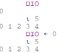
Before defining the final function we need to take an additional consideration. There is a system variable which modifies the origin of the iota function among other things. For example:



In other to make our code independent of the value of IO by using it instead of references to '1' as above.

Defining a function

The final function definition looks like this:




We can use this function as follows:

A quick look at J

In this post I'm going to show a small overview of the J programming language. An example of polynomial multiplication is examined.

J

J is an array programming language derived from APL which means is good for manipulating arrays and matrices. Its syntax and semantics are very different from other languages which makes it an interesting topic for studying.

There's a lot of documentation and examples available from the J software website. Two complete tutorials are "Learning J" by Roger Stokes and "J for C programmers" by Henry Rich.

The J distribution also includes examples and tutorials. The examples will be presented using J's REPL called jconsole.

The example

In order to give an overview of the language I'm going to start from the definition of a function that performs polynomial multiplication and examine how it was constructed.

The function is defined as follows:

polymulti =: dyad : '+/ (((_1 * i. #y) (|. "0 1) ((x (*"_ 0) y) (,"1 1) (((#y) - 1) $ 0))) , 0)'

Writing this example helped me understand some of the J's basic concepts (I'm completely sure there's a better/more efficient way to do this!).

Polynomial multiplication

The basic technique for polynomial multiplication consists on multiplying each term of one of the polynomials by the order and them simply the result. For example:

(4x3 - 23x2 + x + 1)   *   (2x2 - x - 3) 

= ((4x3 - 23x2 + x + 1) * 2x2) + 
  ((4x3 - 23x2 + x + 1) * -x) +
  ((4x3 - 23x2 + x + 1) * -3)

= (8x5 - 46x4 + 2x3 + 2x2) + 
  (-4x4 + 23x3 - x2 - x)  +
  (-12x3 + 69x2 - 3x - 3) 

= (8x5 - 50x4 + 13x3 + 70x2 - 4x - 3)  

Now I'll start creating polymulti from the bottom up to the definition.

1. Defining polynomials

As mentioned above J is a nice language for manipulating arrays. We're going to use J arrays to define polynomials. In fact J supports some operations on arrays as polynomials which will be described bellow.

In order to write a new array literal containing 1,1, -23 and 4 in J we write (here using jconsole):

   1 1 _23 4
1 1 _23 4

As you can see the elements of the array are separated by space. Also negative numbers are prefixed by underscore '_'. This array is going to be used to represent the coefficients of the "(4x³ - 23x² + x + 1)" polynomial.

We're going to define two variables with the polynomials shown above to use them for examples:

   p1 =: 1 1 _23 4
   p2 =: _3 _1 2

Here the '=:' operator is used to bind the specified arrays with p1 and p2.

2. Multiply each element of one of the polynomials

We can proceed to apply the first step in the process which is multiply each element of the second operand by the first operand.

In J we can operate on arrays easily, for example if we want to multiply each element of the above array by a 2 we write:

   1 1 _23 4 * 2
2 2 _46 8

In J the an operation that receives two arguments is called a dyad and a operation that receives only one is called monad. Here we're using the '*' dyad to perform the multiplication.

We cannot directly go and type "p1 * p2" because we will get the following error:

   p1 * p2
|length error
|   p1    *p2

This happens because the length of the two arrays (4 and 3) could not be used to perform the operation. We can apply '*' to a two same size arrays and J will multiply each element. For example:

   p1 * p1
1 1 529 16

Now what I want is to multiply each element of 'p2' by 'p1'. In order to do this we can change the behavior of the '*' dyad by specifying its rank (more details on how to do this can be found in "Verb Execution -- How Rank Is Used (Dyads)") . To change the rank of '*' and say that we want to multiply the complete array on the left for each of the cells of the right array we write (*"_ 0) .For example:

   p1 (*"_ 0) p2
_3 _3  69 _12
_1 _1  23  _4
 2  2 _46   8

By specifying (*"_ 0) we say that the left operand has "infinite rank" (_) which means it will consider the array as single unit.We also say that for the right argument we will consider every cell (by using the 0 rank). Notice that in order to modify the rank we use double quote (") which, in J, doesn't have to paired with another double quote as in most programming languages.

Also you can notice that the result of this operation is an array of arrays, one for each element of the right argument.

2. Sum each element of one of the polynomials

Now that we have an array of polynomials with the result of multiplying the coefficients, we need to change the degree of each of the polynomials. First we need to make more space to increment the degree of the polynomials. We're going to use the ',' dyad which lets you concatenate two arrays. For example:

   p1 , 0 0
1 1 _23 4 0 0

We need to append an array that is the size of the second polynomial minus one. In order to create a new array of this size we use '$' which lets you create an array or matrix by specifying the size and the value of the elements of the new array. For example:

   10 $ 0
0 0 0 0 0 0 0 0 0 0

The size of the array can be obtained with the '#' monad. For example:

   # p1
4

Now we can combine all these elements to resize each array resulting from the multiplication of the coefficients like this:

   (p1 (*"_ 0) p2)
_3 _3  69 _12
_1 _1  23  _4
 2  2 _46   8
    (((#p2) - 1 ) $ 0)
0 0
   (p1 (*"_ 0) p2) (,"1 1) ( ((#p2) - 1 ) $ 0)
_3 _3  69 _12 0 0
_1 _1  23  _4 0 0
 2  2 _46   8 0 0

Here we use (((#p2) - 1 ) $ 0) to generate an array of zeros of the desired size. Then we use (,"1 1) which is the ',' dyad with a modified rank saying that each element of the left matrix (an array) will be concatenated with the second array (since the second argument is a single dimension array we could have said (,"1 _) ).

With the arrays resized we can change the degree of our polynomial array. In order to do this we're going to use the '|.' dyad which let's you rotate an array an specified amount of positions. For example:

 
   1 |.  1 2 3
2 3 1
   _1 |.  1 2 3
3 1 2

As shown in the example, by specifying a positive number the array will be rotated to the left and a negative number to the right.

Now the question is, how to rotate each element of the polynomial array by a different element count? Before showing that we're going to introduce the 'i.' primitive which lets you create an array of with a sequence of numbers for example, to create an array of 10 numbers (starting with 0) we write:

   i. 10
0 1 2 3 4 5 6 7 8 9

We can use this primitive in conjunction with the rotate primitive to say

   m =:    (p1 (*"_ 0) p2) (,"1 1) ( ((#p2) - 1 ) $ 0)
   i. #p2
0 1 2
   _1 * i. #p2
0 _1 _2
   (_1 * i. #p2) (|."0 1) m
_3 _3 69 _12   0 0
 0 _1 _1  23  _4 0
 0  0  2   2 _46 8

As you can see we use the array generated by (_1 * i. #p2) to specify how many positions are we moving. We apply the change the rank of '|.' by saying (|."0 1) which means apply '|.' for each single cell of the left array to each row of the right array.

The previous step generated an array polynomials to be summed. So the only thing left is to generate the final polynomial. In order to do this we use the '+/' dyad which let's use sum the contents of an array. For example:

   +/ 5 3 4 1
13

We can apply +/ to any array and J will do the operation as expected.

   +/ (_1 * i. #p2) (|."0 1) m
_3 _4 70 13 _50 8

As a work around I'm appending a zero row to this matrix, just in case the p2 array is a 0 degree polynomial.

   +/ ((_1 * i. #p2) (|."0 1) m) , 0
_3 _4 70 13 _50 8

And that's it we have the complete process for multiplying the array.

3. Create the function

Now putting all the elements described above we can put together the polynomial multiplication dyad:

polymulti =: dyad : '+/ (((_1 * i. #y) (|. "0 1) ((x (*"_ 0) y) (,"1 1) (((#y) - 1) $ 0))) , 0)'

The 'x' and 'y' names are the implicit names of the left and right operands.

We can use it with any pair of polynomials. For example:

   2 34 3 polymulti 4 3
8 142 114 9
   2 34 3 polymulti 4 0 3
8 136 18 102 9
   2 34 3 polymulti 1
2 34 3

4. Use the polynomials

J already has support for polynomials inside the library. For example by using the 'p.' we can get an evaluation of a given polynomial.

   3 4 5 p. 34
5919
   3 + (4*34) + (5*34*34)
5919
   _2 p. 34
_2
   (5 3 _2 polymulti 3 0 0 _2)
15 9 _6 _10 _6 4
   (5 3 _2 polymulti 3 0 0 _2) p. 3
204

Final words

It was very interesting to read about J. It offers a different perspective on programming which is definitely worth studying. I have to admit it was difficult at the beginning because of the number of concepts to learn ( only a couple are presented in this post) and the syntax . For future posts I'm going to try to explore more J features.